Dressing Boulders for Science

By Jennifer Lamp

This blog post was originally drafted on December 13, but couldn’t be posted until now because the Antarctic fieldwork site lacked an internet connection. Read the team’s previous blog posts here.

Over the last week we made a lot of progress in setting up our weathering and erosion monitoring equipment. On Dec. 6, while Missy finished recording descriptions of our four selected boulders and Kate began taking cosmogenic surface exposure age samples around camp, I wired up the entire acoustic emission arrangement (solar panels, batteries, and monitoring box) together for the first time in Beacon Valley. Thankfully, it’s all working!

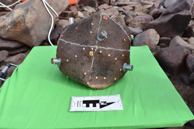
The next few days saw me and Missy in the Scott lab tent, along with Missy’s new favorite toy, the “Big Buddy” propane heater. Unfortunately, setting up the acoustic emission system isn’t as easy as simply attaching sensors to the boulders and hitting “record.” For each boulder, we have to individually determine the wave velocity and the best combination of software settings to reliably record cracking events. We also have to settle on the most appropriate placement of the acoustic emission sensors: for all possible combinations of the six AE sensors attached to each rock, no four can be in-plane with each other, and they have to be adequately spaced to capture cracking in any place on the irregularly-shaped boulders. We will be recording AE hits (a single sensor recording an acoustic emission), AE events (four or more sensors recording the same acoustic emission) and their locations, as well as waveforms. We are primarily interested in AE events, as they help to filter out the noise associated with a single sensor picking up a non-AE signal.

For each boulder, our method to attach the AE sensors is as follows:

1. Create a 3D coordinate system for the boulder.
2. Use chalk to mark the potential placement of the AE sensors. Also mark a few other selected points on the rock for use in determining wave velocity and location error—more on this below.
3. Determine the coordinates of each chalk mark in the coordinate system from Step 1. Due to the lack of a table in the lab tent, this required a lot of crawling around, hunching at odd angles, and multiple bubble levels and rulers.
4. Attach the AE sensors to the boulder using vacuum grease and a lot of masking tape. This is one of the most frustrating parts of the process – the sensors slide around easily in the grease and tape does not like to stick to cold surfaces.
5. Start the AE software, initially using “best-guess” settings. We started with default settings recommended by the manufacturer of the AE monitoring system, which are also similar to what Missy used in her previous AE work.
6. Perform pencil lead breaks (PLBs) to determine the wave velocity. A PLB simulates a microcracking event: we break the tip of a piece of pencil lead at a 30-degree angle from the rock surface near each AE sensor, and at a few other points on the rock. We then log the time it takes for each sensor to record the acoustic emission from the PLB. Since we know the location of each PLB and the distance from the PLB to each AE sensor, we can estimate the rock’s wave velocity, or how quickly the elastic wave generated by the PLB travels through the rock (in millimeters per second).
7. Update the software settings with the average wave velocity found in Step 6.
8. Perform more PLBs, this time comparing the 3D location software’s estimate of the PLB location to its actual location. Repeat multiple times to determine the error in the software location estimate.
9. If there are issues during Steps 6-8—for example, if some sensors don’t record acoustic emission hits during the pencil lead breaks or the software location error is too high—either go back to Step 2 and reposition the AE sensors, or Step 5 and change some of the software settings. Repeat until you can reliably record AE events and their locations.
10. Wipe the vacuum grease off the rock and epoxy each AE sensor in place, using tape to keep it stable as the epoxy cures.

There was a bit of a learning curve, but by the second boulder Missy and I settled on a good system. The lab tent and propane heater have proved crucial to our work – it would be impossible to do all of the sensor attaching out in the wind and cold! We were able to epoxy AE sensors to the first rock on Friday, two more on Saturday, and the last one on Sunday (Dec. 9). While Missy and I were in the lab tent the last few days, Kate continued taking cosmogenic surface exposure age samples from around our campsite. It was awesome of her to get a jump start on this part of the project! After around 2:00 pm on Sunday we all took a break from AE sensors and sampling, and spent a relaxing afternoon in the endurance tent while we let the epoxy cure. We had our first real snowfall on Monday night, and woke up to a beautiful and snowy Beacon Valley.

a" data-cycle-paused="true" data-cycle-prev="#gslideshow_prev" data-cycle-next="#gslideshow_next" data-cycle-pager="#gslideshow_pager" data-cycle-pager-template=" " data-cycle-speed="750" data-cycle-caption="#gslideshow_captions" data-cycle-caption-template="{{cycleCaption}}" > <►>Me posing with “Theresa,” who is covered with masking tape holding AE sensors in place during PLB tests. The “Big Buddy” propane heater is in the back of the photo (and is why we didn’t need to wear our coats/gloves). On the right side of the photo is the pile of sensor cabling we had to work around; this project has proven to be a master class in the importance of cable management. Photo: Missy Eppes

By the end of Tuesday, we were able to additionally attach six thermocouples to each boulder and wire up the Campbell Scientific datalogger that will be recording them. We had planned to attach a surface moisture sensor to each boulder as well, but with six AE sensors and six thermocouples already covering the rock surfaces, we were running out of space. We decided instead to attach the surface moisture sensors to two nearby dolerite boulders which had similar surface characteristics to our four main study boulders. These sensors will tell us when liquid water is present on the rock surfaces, as commonly happens after snow fall events: the dolerites have low albedos, and quickly heat up to over 0°C when the sun is out, melting overlying snow.

On Wednesday and Thursday, we deployed our meteorological station (with sensors to record wind speed/direction, barometric pressure, air temperature/relative humidity, and solar irradiance), helped to carry the rocks that Kate collected for surface exposure dating back to camp (and sampled a few more), and attached guy wire to our solar panels. Earlier in the week we put in a helicopter support request via satellite phone for a trip to the headwall of Mullins Glacier for Friday, Dec. 14. Our plan is for a helicopter to take the three of us and our rock sampling equipment up to a meltwater lake near the glacier headwall, then slowly hike the few kilometers back to our Beacon Valley camp while collecting cosmogenic surface exposure samples along the way. We spent a few hours on Thursday afternoon organizing and packing the samples that Kate collected, and sorting trash and other waste that the helicopter will take back to McMurdo. Tomorrow, Mullins Valley!